Principal Components Analysis and Singular Value Decomposition

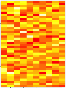
set.seed(12345)
par(mar = rep(0.2, 4))
dataMatrix <- matrix(rnorm(400), nrow = 40)
image(1:10, 1:40, t(dataMatrix)[, nrow(dataMatrix):1])

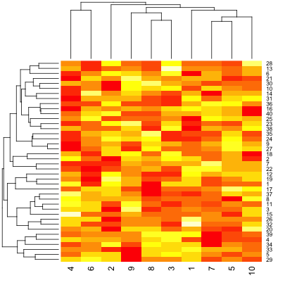
par(mar = rep(0.2, 4))
heatmap(dataMatrix)

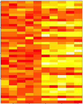
set.seed(678910)
for (i in 1:40) {
    # flip a coin
    coinFlip <- rbinom(1, size = 1, prob = 0.5)
    # if coin is heads add a common pattern to that row
    if (coinFlip) {
        dataMatrix[i, ] <- dataMatrix[i, ] + rep(c(0, 3), each = 5)
    }
}

par(mar = rep(0.2, 4))
image(1:10, 1:40, t(dataMatrix)[, nrow(dataMatrix):1])

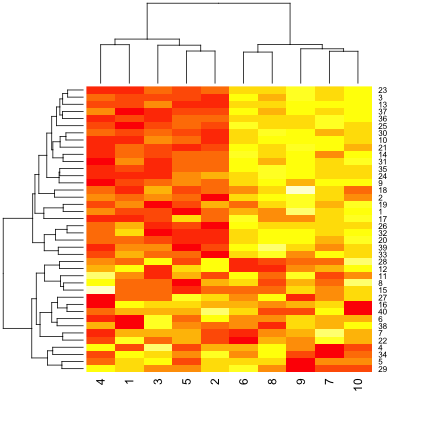
par(mar = rep(0.2, 4))
heatmap(dataMatrix)

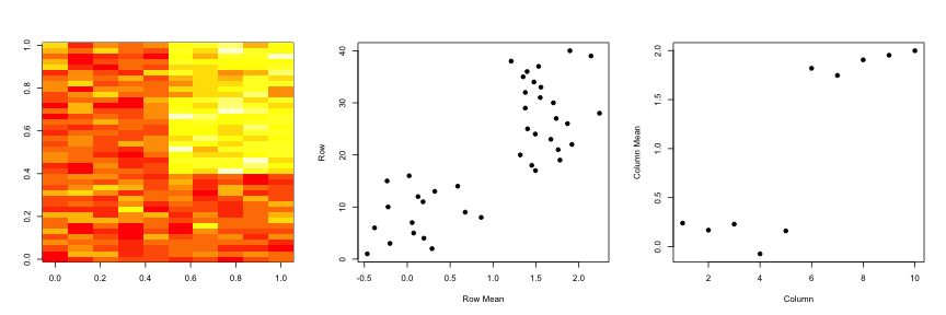
hh <- hclust(dist(dataMatrix))
dataMatrixOrdered <- dataMatrix[hh$order, ]
par(mfrow = c(1, 3))
image(t(dataMatrixOrdered)[, nrow(dataMatrixOrdered):1])
plot(rowMeans(dataMatrixOrdered), 40:1, , xlab = "Row Mean", ylab = "Row", pch = 19)
plot(colMeans(dataMatrixOrdered), xlab = "Column", ylab = "Column Mean", pch = 19)

You have multivariate variables \(X_1,\ldots,X_n\) so \(X_1 = (X_{11},\ldots,X_{1m})\)

• Find a new set of multivariate variables that are uncorrelated and explain as much variance as possible.
• If you put all the variables together in one matrix, find the best matrix created with fewer variables (lower rank) that explains the original data.

The first goal is statistical and the second goal is data compression.

SVD

If \(X\) is a matrix with each variable in a column and each observation in a row then the SVD is a "matrix decomposition"

\[ X = UDV^T\]

where the columns of \(U\) are orthogonal (left singular vectors), the columns of \(V\) are orthogonal (right singular vectors) and \(D\) is a diagonal matrix (singular values).

PCA

The principal components are equal to the right singular values if you first scale (subtract the mean, divide by the standard deviation) the variables.

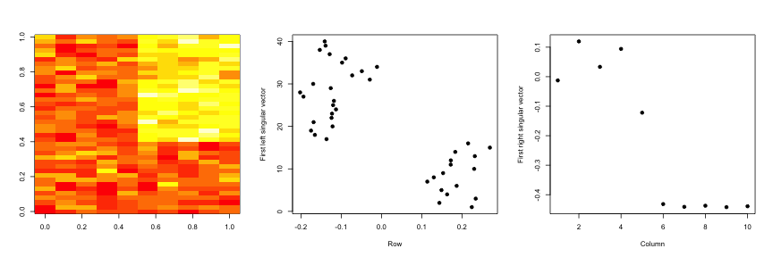
svd1 <- svd(scale(dataMatrixOrdered))
par(mfrow = c(1, 3))
image(t(dataMatrixOrdered)[, nrow(dataMatrixOrdered):1])
plot(svd1$u[, 1], 40:1, , xlab = "Row", ylab = "First left singular vector", 
    pch = 19)
plot(svd1$v[, 1], xlab = "Column", ylab = "First right singular vector", pch = 19)

par(mfrow = c(1, 2))
plot(svd1$d, xlab = "Column", ylab = "Singular value", pch = 19)
plot(svd1$d^2/sum(svd1$d^2), xlab = "Column", ylab = "Prop. of variance explained", 
    pch = 19)

svd1 <- svd(scale(dataMatrixOrdered))
pca1 <- prcomp(dataMatrixOrdered, scale = TRUE)
plot(pca1$rotation[, 1], svd1$v[, 1], pch = 19, xlab = "Principal Component 1", 
    ylab = "Right Singular Vector 1")
abline(c(0, 1))

constantMatrix <- dataMatrixOrdered*0
for(i in 1:dim(dataMatrixOrdered)[1]){constantMatrix[i,] <- rep(c(0,1),each=5)}
svd1 <- svd(constantMatrix)
par(mfrow=c(1,3))
image(t(constantMatrix)[,nrow(constantMatrix):1])
plot(svd1$d,xlab="Column",ylab="Singular value",pch=19)
plot(svd1$d^2/sum(svd1$d^2),xlab="Column",ylab="Prop. of variance explained",pch=19)

set.seed(678910)
for (i in 1:40) {
    # flip a coin
    coinFlip1 <- rbinom(1, size = 1, prob = 0.5)
    coinFlip2 <- rbinom(1, size = 1, prob = 0.5)
    # if coin is heads add a common pattern to that row
    if (coinFlip1) {
        dataMatrix[i, ] <- dataMatrix[i, ] + rep(c(0, 5), each = 5)
    }
    if (coinFlip2) {
        dataMatrix[i, ] <- dataMatrix[i, ] + rep(c(0, 5), 5)
    }
}
hh <- hclust(dist(dataMatrix))
dataMatrixOrdered <- dataMatrix[hh$order, ]

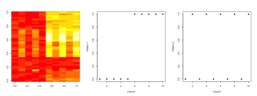
svd2 <- svd(scale(dataMatrixOrdered))
par(mfrow = c(1, 3))
image(t(dataMatrixOrdered)[, nrow(dataMatrixOrdered):1])
plot(rep(c(0, 1), each = 5), pch = 19, xlab = "Column", ylab = "Pattern 1")
plot(rep(c(0, 1), 5), pch = 19, xlab = "Column", ylab = "Pattern 2")

svd2 <- svd(scale(dataMatrixOrdered))
par(mfrow = c(1, 3))
image(t(dataMatrixOrdered)[, nrow(dataMatrixOrdered):1])
plot(svd2$v[, 1], pch = 19, xlab = "Column", ylab = "First right singular vector")
plot(svd2$v[, 2], pch = 19, xlab = "Column", ylab = "Second right singular vector")

svd1 <- svd(scale(dataMatrixOrdered))
par(mfrow = c(1, 2))
plot(svd1$d, xlab = "Column", ylab = "Singular value", pch = 19)
plot(svd1$d^2/sum(svd1$d^2), xlab = "Column", ylab = "Percent of variance explained", 
    pch = 19)

dataMatrix2 <- dataMatrixOrdered
## Randomly insert some missing data
dataMatrix2[sample(1:100, size = 40, replace = FALSE)] <- NA
svd1 <- svd(scale(dataMatrix2))  ## Doesn't work!

## Error: infinite or missing values in 'x'

library(impute)  ## Available from http://bioconductor.org
dataMatrix2 <- dataMatrixOrdered
dataMatrix2[sample(1:100,size=40,replace=FALSE)] <- NA
dataMatrix2 <- impute.knn(dataMatrix2)$data
svd1 <- svd(scale(dataMatrixOrdered)); svd2 <- svd(scale(dataMatrix2))
par(mfrow=c(1,2)); plot(svd1$v[,1],pch=19); plot(svd2$v[,1],pch=19)

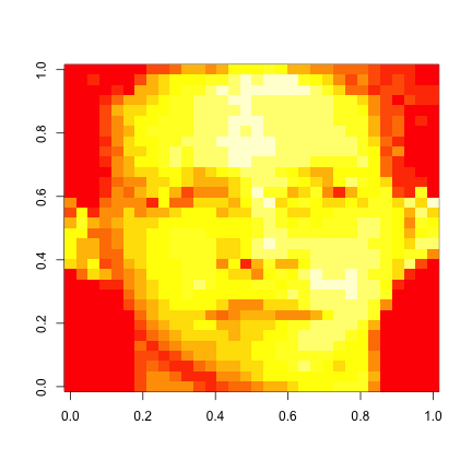
load("data/face.rda")
image(t(faceData)[, nrow(faceData):1])

svd1 <- svd(scale(faceData))
plot(svd1$d^2/sum(svd1$d^2), pch = 19, xlab = "Singular vector", ylab = "Variance explained")

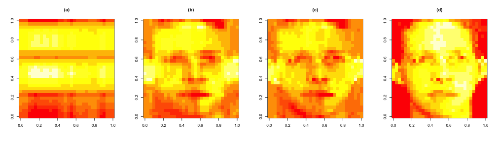
svd1 <- svd(scale(faceData))
## Note that %*% is matrix multiplication

# Here svd1$d[1] is a constant
approx1 <- svd1$u[, 1] %*% t(svd1$v[, 1]) * svd1$d[1]

# In these examples we need to make the diagonal matrix out of d
approx5 <- svd1$u[, 1:5] %*% diag(svd1$d[1:5]) %*% t(svd1$v[, 1:5])
approx10 <- svd1$u[, 1:10] %*% diag(svd1$d[1:10]) %*% t(svd1$v[, 1:10])

par(mfrow = c(1, 4))
image(t(approx1)[, nrow(approx1):1], main = "(a)")
image(t(approx5)[, nrow(approx5):1], main = "(b)")
image(t(approx10)[, nrow(approx10):1], main = "(c)")
image(t(faceData)[, nrow(faceData):1], main = "(d)")  ## Original data

• Scale matters
• PC's/SV's may mix real patterns
• Can be computationally intensive
• Advanced data analysis from an elementary point of view
• Elements of statistical learning
• Alternatives
  • Factor analysis
  • Independent components analysis
  • Latent semantic analysis