Introduction to the R Language

Scoping Rules

Roger D. Peng, Associate Professor of Biostatistics
Johns Hopkins Bloomberg School of Public Health

A Diversion on Binding Values to Symbol

How does R know which value to assign to which symbol? When I type

> lm <- function(x) { x * x }
> lm
function(x) { x * x }

how does R know what value to assign to the symbol lm? Why doesn’t it give it the value of lm that is in the stats package?
A Diversion on Binding Values to Symbol

When R tries to bind a value to a symbol, it searches through a series of environments to find the appropriate value. When you are working on the command line and need to retrieve the value of an R object, the order is roughly

  1. Search the global environment for a symbol name matching the one requested.
  2. Search the namespaces of each of the packages on the search list

The search list can be found by using the search function.

> search()
[1] ".GlobalEnv"        "package:stats"     "package:graphics"
[4] "package:grDevices" "package:utils"     "package:datasets"
[7] "package:methods"   "Autoloads"         "package:base"

Binding Values to Symbol

  • The global environment or the user’s workspace is always the first element of the search list and the base package is always the last.
  • The order of the packages on the search list matters!
  • User’s can configure which packages get loaded on startup so you cannot assume that there will be a set list of packages available.
  • When a user loads a package with library the namespace of that package gets put in position 2 of the search list (by default) and everything else gets shifted down the list.
  • Note that R has separate namespaces for functions and non-functions so it’s possible to have an object named c and a function named c.

Scoping Rules

The scoping rules for R are the main feature that make it different from the original S language.

  • The scoping rules determine how a value is associated with a free variable in a function
  • R uses lexical scoping or static scoping. A common alternative is dynamic scoping.
  • Related to the scoping rules is how R uses the search list to bind a value to a symbol
  • Lexical scoping turns out to be particularly useful for simplifying statistical computations

Lexical Scoping

Consider the following function.

f <- function(x, y) {
        x^2 + y / z
}

This function has 2 formal arguments x and y. In the body of the function there is another symbol z. In this case z is called a free variable. The scoping rules of a language determine how values are assigned to free variables. Free variables are not formal arguments and are not local variables (assigned insided the function body).

Lexical Scoping

Lexical scoping in R means that

the values of free variables are searched for in the environment in which the function was defined.

What is an environment?

  • An environment is a collection of (symbol, value) pairs, i.e. x is a symbol and 3.14 might be its value.
  • Every environment has a parent environment; it is possible for an environment to have multiple “children”
  • the only environment without a parent is the empty environment
  • A function + an environment = a closure or function closure.

Lexical Scoping

Searching for the value for a free variable:

  • If the value of a symbol is not found in the environment in which a function was defined, then the search is continued in the parent environment.
  • The search continues down the sequence of parent environments until we hit the top-level environment; this usually the global environment (workspace) or the namespace of a package.
  • After the top-level environment, the search continues down the search list until we hit the empty environment. If a value for a given symbol cannot be found once the empty environment is arrived at, then an error is thrown.

Lexical Scoping

Why does all this matter?

  • Typically, a function is defined in the global environment, so that the values of free variables are just found in the user’s workspace
  • This behavior is logical for most people and is usually the “right thing” to do
  • However, in R you can have functions defined inside other functions
    • Languages like C don’t let you do this
  • Now things get interesting — In this case the environment in which a function is defined is the body of another function!

Lexical Scoping

make.power <- function(n) {
        pow <- function(x) {
                x^n 
        }
        pow 
}

This function returns another function as its value.

> cube <- make.power(3)
> square <- make.power(2)
> cube(3)
[1] 27
> square(3)
[1] 9

Exploring a Function Closure

What’s in a function’s environment?

> ls(environment(cube))
[1] "n"   "pow"
> get("n", environment(cube))
[1] 3

> ls(environment(square))
[1] "n"   "pow"
> get("n", environment(square))
[1] 2

Lexical vs. Dynamic Scoping

y <- 10

f <- function(x) {
        y <- 2
        y^2 + g(x)
}

g <- function(x) { 
        x*y
}

What is the value of

f(3)

Lexical vs. Dynamic Scoping

  • With lexical scoping the value of y in the function g is looked up in the environment in which the function was defined, in this case the global environment, so the value of y is 10.
  • With dynamic scoping, the value of y is looked up in the environment from which the function was called (sometimes referred to as the calling environment).
    • In R the calling environment is known as the parent frame
  • So the value of y would be 2.

Lexical vs. Dynamic Scoping

When a function is defined in the global environment and is subsequently called from the global environment, then the defining environment and the calling environment are the same. This can sometimes give the appearance of dynamic scoping.

> g <- function(x) { 
+ a <- 3
+ x+a+y 
+ }
> g(2)
Error in g(2) : object "y" not found
> y <- 3
> g(2)
[1] 8

Other Languages

Other languages that support lexical scoping

  • Scheme
  • Perl
  • Python
  • Common Lisp (all languages converge to Lisp)

Consequences of Lexical Scoping

  • In R, all objects must be stored in memory
  • All functions must carry a pointer to their respective defining environments, which could be anywhere
  • In S-PLUS, free variables are always looked up in the global workspace, so everything can be stored on the disk because the “defining environment” of all functions is the same.

Application: Optimization

Why is any of this information useful?

  • Optimization routines in R like optim, nlm, and optimize require you to pass a function whose argument is a vector of parameters (e.g. a log-likelihood)
  • However, an object function might depend on a host of other things besides its parameters (like data)
  • When writing software which does optimization, it may be desirable to allow the user to hold certain parameters fixed

Maximizing a Normal Likelihood

Write a “constructor” function

make.NegLogLik <- function(data, fixed=c(FALSE,FALSE)) {
        params <- fixed
        function(p) {
                params[!fixed] <- p
                mu <- params[1]
                sigma <- params[2]
                a <- -0.5*length(data)*log(2*pi*sigma^2)
                b <- -0.5*sum((data-mu)^2) / (sigma^2)
                -(a + b)
        } 
}

Note: Optimization functions in R minimize functions, so you need to use the negative log-likelihood.

Maximizing a Normal Likelihood

> set.seed(1); normals <- rnorm(100, 1, 2)
> nLL <- make.NegLogLik(normals)
> nLL
function(p) {
                params[!fixed] <- p
                mu <- params[1]
                sigma <- params[2]
                a <- -0.5*length(data)*log(2*pi*sigma^2)
                b <- -0.5*sum((data-mu)^2) / (sigma^2)
                -(a + b)
        }
<environment: 0x165b1a4>
> ls(environment(nLL))
[1] "data"   "fixed"  "params"

Estimating Parameters

> optim(c(mu = 0, sigma = 1), nLL)$par
      mu    sigma
1.218239 1.787343

Fixing σ = 2

> nLL <- make.NegLogLik(normals, c(FALSE, 2))
> optimize(nLL, c(-1, 3))$minimum
[1] 1.217775

Fixing μ = 1

> nLL <- make.NegLogLik(normals, c(1, FALSE))
> optimize(nLL, c(1e-6, 10))$minimum
[1] 1.800596

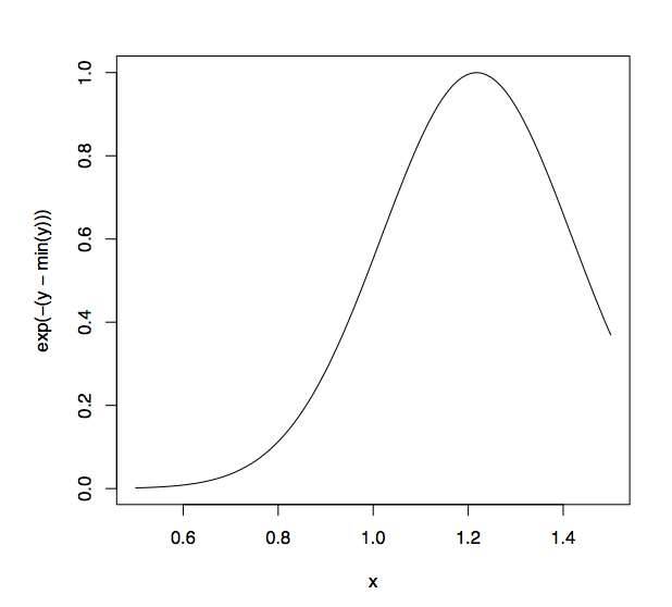
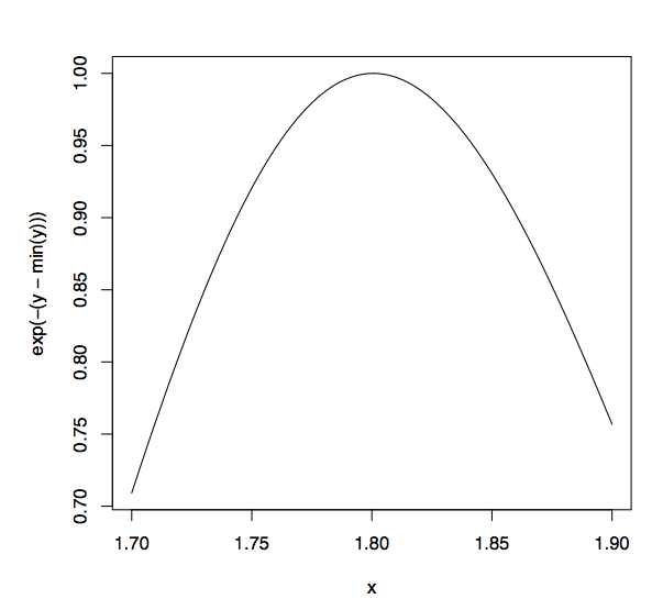
Plotting the Likelihood

nLL <- make.NegLogLik(normals, c(1, FALSE))
x <- seq(1.7, 1.9, len = 100)
y <- sapply(x, nLL)
plot(x, exp(-(y - min(y))), type = "l")

nLL <- make.NegLogLik(normals, c(FALSE, 2))
x <- seq(0.5, 1.5, len = 100)
y <- sapply(x, nLL)
plot(x, exp(-(y - min(y))), type = "l")

Plotting the Likelihood

Plotting the Likelihood

Lexical Scoping Summary

  • Objective functions can be “built” which contain all of the necessary data for evaluating the function
  • No need to carry around long argument lists — useful for interactive and exploratory work.
  • Code can be simplified and cleand up
  • Reference: Robert Gentleman and Ross Ihaka (2000). “Lexical Scope and Statistical Computing,” JCGS, 9, 491–508.